import numpy as np
import pandas as pd
from matplotlib.pyplot import subplots
from statsmodels.datasets import get_rdataset
import sklearn.model_selection as skm
from ISLP import load_data , confusion_table
from ISLP.models import ModelSpec as MS1. imports
from sklearn.tree import (DecisionTreeClassifier as DTC ,
                          DecisionTreeRegressor as DTR, plot_tree, export_text)
from sklearn.metrics import (accuracy_score, log_loss)
from sklearn.ensemble import (RandomForestRegressor as RF, GradientBoostingRegressor as GBR)
from ISLP.bart import BART
2. Data
Carseats = load_data('Carseats')
High = np.where(Carseats.Sales > 8, "Yes", "No")
3. 단순 나무 모형 적용
model = MS(Carseats.columns.drop('Sales'), intercept=False)
D = model.fit_transform(Carseats)
feature_names = list(D.columns)
X = np.asarray(D)

clf = DTC(criterion='entropy', max_depth=3, random_state=0)
# 깊이는 3으로, 손실함수는 엔트로피 이용
clf.fit(X, High)
DecisionTreeClassifier(criterion='entropy', max_depth=3, random_state=0)In a Jupyter environment, please rerun this cell to show the HTML representation or trust the notebook.
On GitHub, the HTML representation is unable to render, please try loading this page with nbviewer.org.
DecisionTreeClassifier(criterion='entropy', max_depth=3, random_state=0)
- 분류 문제에서 예측오차, 손실함수의 값, 의사결정 나무 확인
accuracy_score(High , clf.predict(X))0.79- Residual deviance: $ -2 m k n{mk} {mk} $
resid_dev = np.sum(log_loss(High , clf.predict_proba(X)))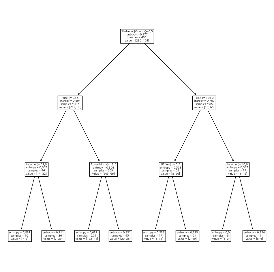
resid_dev0.4710647062649358ax = subplots(figsize=(12,12))[1]
plot_tree(clf, feature_names=feature_names, ax=ax);
print(export_text(clf, feature_names=feature_names, show_weights=True))
# weights: 0과 1의 비중|--- ShelveLoc[Good] <= 0.50
| |--- Price <= 92.50
| | |--- Income <= 57.00
| | | |--- weights: [7.00, 3.00] class: No
| | |--- Income > 57.00
| | | |--- weights: [7.00, 29.00] class: Yes
| |--- Price > 92.50
| | |--- Advertising <= 13.50
| | | |--- weights: [183.00, 41.00] class: No
| | |--- Advertising > 13.50
| | | |--- weights: [20.00, 25.00] class: Yes
|--- ShelveLoc[Good] > 0.50
| |--- Price <= 135.00
| | |--- US[Yes] <= 0.50
| | | |--- weights: [6.00, 11.00] class: Yes
| | |--- US[Yes] > 0.50
| | | |--- weights: [2.00, 49.00] class: Yes
| |--- Price > 135.00
| | |--- Income <= 46.00
| | | |--- weights: [6.00, 0.00] class: No
| | |--- Income > 46.00
| | | |--- weights: [5.00, 6.00] class: Yes
- Validation error 확인
validation = skm.ShuffleSplit(n_splits=1, test_size=200, random_state=0)
results = skm.cross_validate(clf, D, High, cv=validation)
results['test_score']array([0.685])- 두 개의 데이터셋으로 쪼개서 훈련과 평가 진행
(X_train, X_test, High_train, High_test) = skm.train_test_split(X, High, test_size=0.5, random_state=0)
clf = DTC(criterion='entropy', random_state=0)
clf.fit(X_train, High_train)
accuracy_score(High_test, clf.predict(X_test))0.735- 훈련 데이터에서 CV로 최적의 pruning 을 선택
ccp_path = clf.cost_complexity_pruning_path(X_train, High_train)
kfold = skm.KFold(10, random_state=1, shuffle=True)
grid = skm.GridSearchCV(clf, {'ccp_alpha': ccp_path.ccp_alphas}, refit=True,cv=kfold,
scoring='accuracy')
grid.fit(X_train, High_train)
grid.best_score_0.685- CV로 선택된 최적의 의사결정나무를 그림
ax = subplots(figsize=(12, 12))[1]
best_ = grid.best_estimator_
plot_tree(best_, feature_names=feature_names, ax=ax);
best_.tree_.n_leaves
30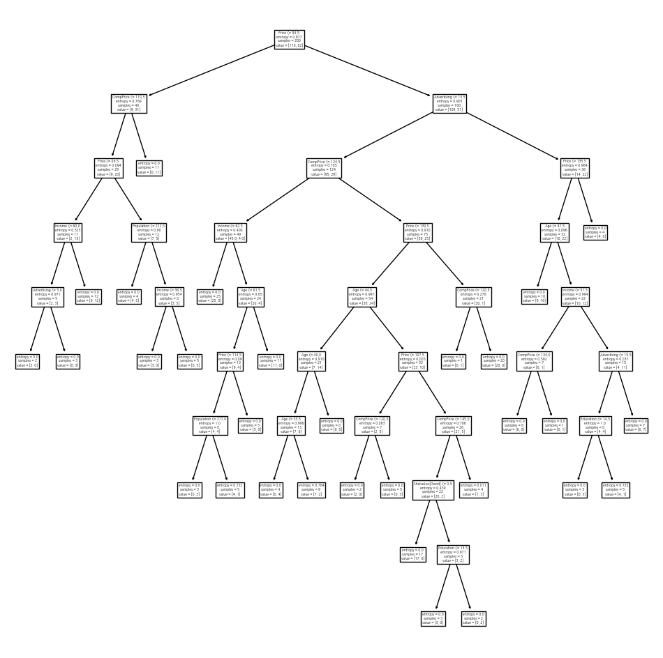
- 훈련 데이터에서 모형을 구축하고 평가 데이터에서 혼동행렬을 봄
print(accuracy_score(High_test, best_.predict(X_test)))
confusion = confusion_table(best_.predict(X_test), High_test)
print(confusion)
0.72
Truth No Yes
Predicted
No 94 32
Yes 24 50- 보스턴 데이터 로딩 및 의사결정나무(회귀분석) 분석 진행
Boston = load_data("Boston")
model = MS(Boston.columns.drop('medv'), intercept=False)
D = model.fit_transform(Boston)
feature_names = list(D.columns)
X = np.asarray(D)
(X_train, X_test, y_train, y_test) = skm.train_test_split(X, Boston['medv'],test_size=0.3, random_state=0)
reg = DTR(max_depth=3)
reg.fit(X_train , y_train)
ax = subplots(figsize=(12,12))[1]
plot_tree(reg, feature_names=feature_names, ax=ax);
- CV를 통한 최적의 pruning을 진행
ccp_path = reg.cost_complexity_pruning_path(X_train , y_train)
kfold = skm.KFold(5, shuffle=True, random_state =10)
grid = skm.GridSearchCV(reg, {'ccp_alpha': ccp_path.ccp_alphas}, refit=True, cv=kfold,
       scoring='neg_mean_squared_error')
G = grid.fit(X_train, y_train)
best_ = grid.best_estimator_
np.mean((y_test - best_.predict(X_test))**2)28.06985754975404ax = subplots(figsize=(12,12))[1]
plot_tree(G.best_estimator_, feature_names=feature_names, ax=ax);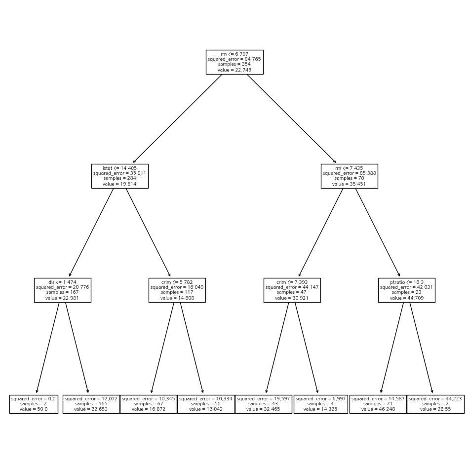
4. RF(Random Forests)
- 보스턴 데이터에 대한 랜덤 포레스트 진행
bag_boston = RF(max_features=X_train.shape[1], random_state=0)
bag_boston.fit(X_train , y_train)
RandomForestRegressor(max_features=12, random_state=0)In a Jupyter environment, please rerun this cell to show the HTML representation or trust the notebook.
On GitHub, the HTML representation is unable to render, please try loading this page with nbviewer.org.
RandomForestRegressor(max_features=12, random_state=0)
- 예측값과 산점도를 통해서 정확도를 확인, 예측오차를 계산
ax = subplots(figsize=(8,8))[1]
y_hat_bag = bag_boston.predict(X_test)
ax.scatter(y_hat_bag , y_test)
np.mean((y_test - y_hat_bag)**2)
14.634700151315787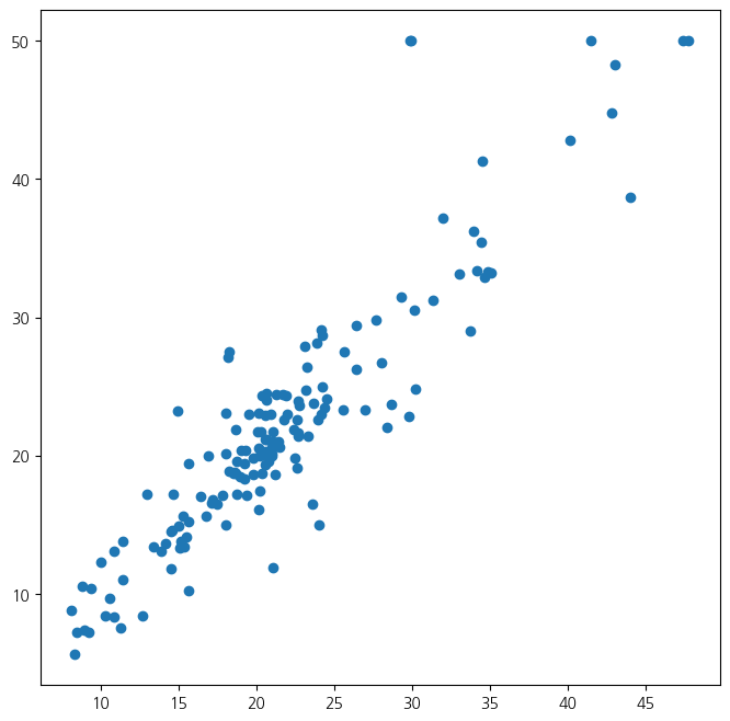
- 랜덤 포레스트에서 사용하는 변수의 개수를 조정
bag_boston = RF(max_features=X_train.shape[1],
n_estimators=500, random_state=0).fit(X_train , y_train)
y_hat_bag = bag_boston.predict(X_test)
print(np.mean((y_test - y_hat_bag)**2))

# usinbg sqrt(p) variables
RF_boston = RF(max_features=6, random_state=0).fit(X_train , y_train)
y_hat_RF = RF_boston.predict(X_test)
print(np.mean((y_test - y_hat_RF)**2))
14.605662565263161
20.04276446710527- 변수의 중요도를 의미하는 importance를 확인
feature_imp = pd.DataFrame( {'importance':RF_boston.feature_importances_}, index=feature_names)
print(feature_imp.sort_values(by='importance', ascending=False))
importance
lstat 0.356203
rm 0.332163
ptratio 0.067270
crim 0.055404
indus 0.053851
dis 0.041582
nox 0.035225
tax 0.025355
age 0.021506
rad 0.004784
chas 0.004203
zn 0.002454- 그래디언트 부스팅을 진행
- 동원된 의사결정나무는 5000개, 최대 깊이는 3, 학습률은 0.001
boost_boston = GBR(n_estimators=50000, learning_rate =0.001, max_depth=3,
random_state=0)
boost_boston.fit(X_train , y_train)

test_error = np.zeros_like(boost_boston.train_score_)
for idx , y_ in enumerate(boost_boston.staged_predict(X_test)):
  test_error[idx] = np.mean((y_test - y_)**2)
plot_idx = np.arange(boost_boston.train_score_.shape[0])
ax = subplots(figsize=(8,8))[1]
ax.plot(plot_idx, boost_boston.train_score_, 'b', label='Training')

ax.plot(plot_idx, test_error, 'r', label='Test')
ax.legend();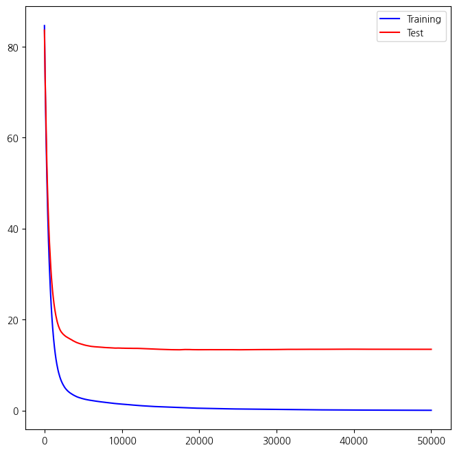
- 위 그림에서 단계 진행에 따른 훈련과 평가 예측오차를 확인, 아래는 예측오차 계산
y_hat_boost = boost_boston.predict(X_test)
np.mean((y_test - y_hat_boost)**2)13.461677803903655- 학습률 조정에 따른 예측오차
boost_boston = GBR(n_estimators=5000, learning_rate=0.2, max_depth=3,random_state=0)
boost_boston.fit(X_train, y_train)
y_hat_boost = boost_boston.predict(X_test);
np.mean((y_test - y_hat_boost)**2)14.5015145537195655. 베이지안 의사결정나무
- 평가 데이터에서 예측오차 확인
bart_boston = BART(random_state=0, burnin=5, ndraw=15)
# burn-in: 앞의 몇 개를 잘라냄, ndraw: 몇 개의 연쇄 샘플링을 할지 경정
bart_boston.fit(X_train , y_train)

yhat_test = bart_boston.predict(X_test.astype(np.float32))
np.mean((y_test - yhat_test)**2)22.145009458109225- 변수의 중요도
var_inclusion = pd.Series(bart_boston.variable_inclusion_.mean(0), index=D.columns)
print(var_inclusion)
crim 26.933333
zn 27.866667
indus 26.466667
chas 22.466667
nox 26.600000
rm 29.800000
age 22.733333
dis 26.466667
rad 23.666667
tax 24.133333
ptratio 24.266667
lstat 31.000000
dtype: float64