12. GR

Author

이상민

Published

June 2, 2025

set.seed(11)
rbinom(2500, 1, 0.5) -> ipp 
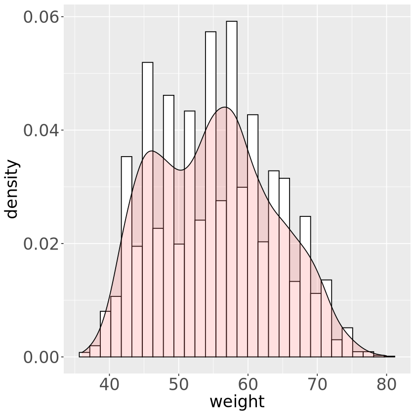
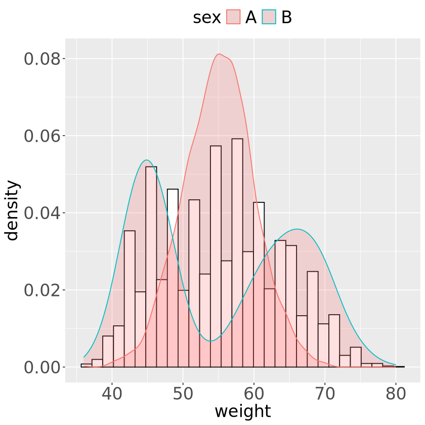
df <- data.frame(
sex=factor(rep(c("A", "B"), each=2500)), weight=round(c(rnorm(2500, mean=55, sd=5),
ipp* rnorm(2500, mean=65, sd=5)                                                     + (1-ipp)*rnorm(2500, mean=45, sd=3) ) ))
head(df) ; tail(df)
A data.frame: 6 × 2
sex weight
<fct> <dbl>
1 A 56
2 A 64
3 A 57
4 A 48
5 A 55
6 A 57
A data.frame: 6 × 2
sex weight
<fct> <dbl>
4995 B 65
4996 B 45
4997 B 68
4998 B 66
4999 B 47
5000 B 63
library(ggplot2)
ggplot(df, aes(x=weight)) + geom_histogram()
library(ggplot2)
ggplot(df, aes(x=weight)) + geom_histogram() + geom_histogram(color='blue', fill='orange')
`stat_bin()` using `bins = 30`. Pick better value with `binwidth`.

library(ggplot2)
ggplot(df, aes(x=weight)) + geom_histogram(binwidth=10, color="blue", fill="orange")
library(ggplot2)
ggplot(df, aes(x=weight)) + geom_histogram(binwidth=0.1, color="blue", fill="orange")

ggplot(df, aes(x=weight)) + geom_histogram(aes(y=..density..), 
  colour="black", fill="white")+ geom_density(alpha=.2, fill="#FF6666") + 
  # geom_histogram(position="dodge")+ 
  theme(legend.position="top") + theme(axis.title = element_text(size=20),
  legend.title = element_text(size=20), 
  legend.text = element_text(size=20), axis.text = element_text(size=20))
Warning message:
“The dot-dot notation (`..density..`) was deprecated in ggplot2 3.4.0.
ℹ Please use `after_stat(density)` instead.”
`stat_bin()` using `bins = 30`. Pick better value with `binwidth`.

ggplot(df, aes(x=weight, color=sex, fill=sex)) + 
  geom_histogram(aes(y=..density..), colour="black", fill="white")+ 
  geom_density(alpha= 0.2, fill="#FF6666") +
  theme(legend.position="top") + 
  theme(axis.title = element_text(size=20), legend.title = element_text(size=20),
  legend.text = element_text(size=20), axis.text = element_text(size=20))
`stat_bin()` using `bins = 30`. Pick better value with `binwidth`.

head(OrchardSprays)
ggplot(OrchardSprays, aes(x=factor(treatment), y=decrease, fill=factor(treatment)))+
  geom_violin(adjust=0.5, scale='width', color = rainbow(1))+
  geom_boxplot(size=1, width=0.5)+ theme_minimal()
A data.frame: 6 × 4
decrease rowpos colpos treatment
<dbl> <dbl> <dbl> <fct>
1 57 1 1 D
2 95 2 1 E
3 8 3 1 B
4 69 4 1 H
5 92 5 1 G
6 90 6 1 F

data(VADeaths) 
# par(mfrow=c(1,1))
colnames(VADeaths) = c('rM','rF','uM','uF') 
barplot(round(VADeaths[1,]), col=2:5, border='white', ylim=c(0,25), main= 'VADeaths (50-54)')

require(ggplot2) ; data(UCBAdmissions) ; 
str(UCBAdmissions) 
addmargins(apply(UCBAdmissions, c(2,1), sum))
require(graphics) 
mosaicplot(apply(UCBAdmissions, c(2,1), sum),
           color=c('gray','red'), main ='UC Berkeley Admissions' )
 'table' num [1:2, 1:2, 1:6] 512 313 89 19 353 207 17 8 120 205 ...
 - attr(*, "dimnames")=List of 3
  ..$ Admit : chr [1:2] "Admitted" "Rejected"
  ..$ Gender: chr [1:2] "Male" "Female"
  ..$ Dept  : chr [1:6] "A" "B" "C" "D" ...
A matrix: 3 × 3 of type dbl
Admitted Rejected Sum
Male 1198 1493 2691
Female 557 1278 1835
Sum 1755 2771 4526

require(graphics) 
mosaicplot(apply(UCBAdmissions, c(2,1), sum), 
  color=c('gray','red'), main ='UC Berkeley Admissions' )
mosaicplot(~Dept+Gender+Admit, data=UCBAdmissions, 
           color=c('gray','red'), dir = c('v','v','h'), 
           main ='UC Berkeley Admissions' )

library(treemap) 
data(GNI2014) ; str(GNI2014)
treemap(GNI2014, index = c('continent','iso3'), 
        vSize='population', vColor='GNI', type='value')
'data.frame':   188 obs. of  5 variables:
 $ iso3      : chr  "BMU" "NOR" "QAT" "CHE" ...
 $ country   : chr  "Bermuda" "Norway" "Qatar" "Switzerland" ...
 $ continent : Factor w/ 8 levels "Africa","Antarctica",..: 5 4 3 4 3 4 6 4 4 5 ...
 $ population: num  67837 4676305 833285 7604467 559846 ...
 $ GNI       : int  106140 103630 92200 88120 76270 75990 64540 61610 61310 55200 ...

GNI2014$GNI.total = GNI2014$GNI * GNI2014$population
GNI2014.a = aggregate(GNI2014[,4:6], by = list(GNI2014$continent), sum) 
GNI2014.a$GNI = GNI2014.a$GNI.total/GNI2014.a$population 
treemap(GNI2014.a, index = c('Group.1'), vSize='population', 
        vColor='GNI', type='value' )