1. library
library (tidyverse) # 데이터 처리 및 시각화 library (caret) # 데이터 전처리, 분할, 평가 library (class) # KNN 분류 함수 library (ggplot2)library (gridExtra)
Warning message:
“Your system is mis-configured: ‘/var/db/timezone/localtime’ is not a symlink”
Warning message:
“‘/var/db/timezone/localtime’ is not identical to any known timezone file”
── Attaching core tidyverse packages ───────────────────────────────────────── tidyverse 2.0.0 ──
✔ dplyr     1.1.4     ✔ readr     2.1.5
✔ forcats   1.0.0     ✔ stringr   1.5.1
✔ ggplot2   3.5.1     ✔ tibble    3.2.1
✔ lubridate 1.9.3     ✔ tidyr     1.3.1
✔ purrr     1.0.2
── Conflicts ─────────────────────────────────────────────────────────── tidyverse_conflicts() ──
✖ dplyr::filter() masks stats::filter()
✖ dplyr::lag()    masks stats::lag()
ℹ Use the conflicted package (<http://conflicted.r-lib.org/>) to force all conflicts to become errors
Loading required package: lattice


Attaching package: ‘caret’


The following object is masked from ‘package:purrr’:

    lift


Attaching package: ‘gridExtra’


The following object is masked from ‘package:dplyr’:

    combine
2. Data
<- read.csv ("fake_bills.csv" , sep = ";" )
3. 전처리
- 결측값 제거
- 목표변수 범주형으로 변환
$ is_genuine <- as.factor (dt$ is_genuine)
- X,y분리
<- dt %>% select (- is_genuine)<- dt$ is_genuine
- 표준화
<- preProcess (X, method = c ("center" , "scale" ))<- predict (pre_proc, X)
4. 적합
- 반복 설정
<- 100 <- nrow (X_scaled)<- round (0.7 * N)<- 1 : 100 <- matrix (NA , nrow = T, ncol = length (k_range))
- 반복 : train/test 나눠서 k별 정확도 저장
for (t in 1 : T) {set.seed (t)<- sample (1 : N, n_train, replace = FALSE )<- setdiff (1 : N, train_idx)<- X_scaled[train_idx, ]<- X_scaled[test_idx, ]<- y[train_idx]<- y[test_idx]for (k in k_range) {<- knn (train = x_train, test = x_test, cl = y_train, k = k)<- mean (pred == y_test)
- 평균 정확도 계산
<- colMeans (acc_matrix, na.rm = TRUE )<- data.frame (k = k_range, Accuracy = avg_acc)
- 시각화
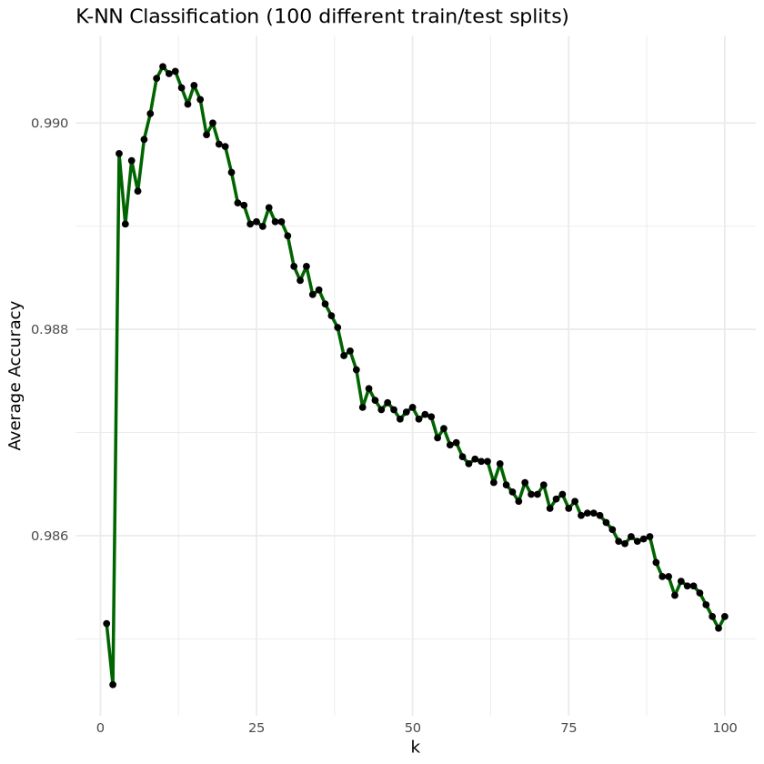
ggplot (results, aes (x = k, y = Accuracy)) + geom_line (color = "darkgreen" , size = 1 ) + geom_point (color = "black" ) + labs (title = "K-NN Classification (100 different train/test splits)" ,x = "k" ,y = "Average Accuracy" ) + theme_minimal ()
Warning message:
“Using `size` aesthetic for lines was deprecated in ggplot2 3.4.0.
ℹ Please use `linewidth` instead.”
- 최적의 k
<- results$ k[which.max (results$ Accuracy)]cat ("★ 최적의 k 값:" , best_k, " \n " )
- 최종 예측 비교
set.seed (999 )<- sample (1 : N, n_train, replace = FALSE )<- setdiff (1 : N, train_index)<- X_scaled[train_index, ]<- X_scaled[test_index, ]<- y[train_index]<- y[test_index]
- 최적 k 예측
<- knn (train = x_train, test = x_test, cl = y_train, k = best_k)
- k=100 예측
<- knn (train = x_train, test = x_test, cl = y_train, k = 100 )
- 정확도 비교
<- mean (best_pred == y_test)<- mean (k100_pred == y_test)cat ("✔️ Best k (" , best_k, ") 정확도:" , round (acc_best * 100 , 2 ), "% \n " )cat ("✔️ k = 100 정확도:" , round (acc_k100 * 100 , 2 ), "% \n " )
✔️ Best k ( 10 ) 정확도: 99.32 %
✔️ k = 100 정확도: 98.63 %
- 혼동행렬 출력
cat (" \n ▶ 혼동행렬 (Best k): \n " )print (confusionMatrix (best_pred, y_test))cat (" \n ▶ 혼동행렬 (k = 100): \n " )print (confusionMatrix (k100_pred, y_test))
▶ 혼동행렬 (Best k):
Confusion Matrix and Statistics
Reference
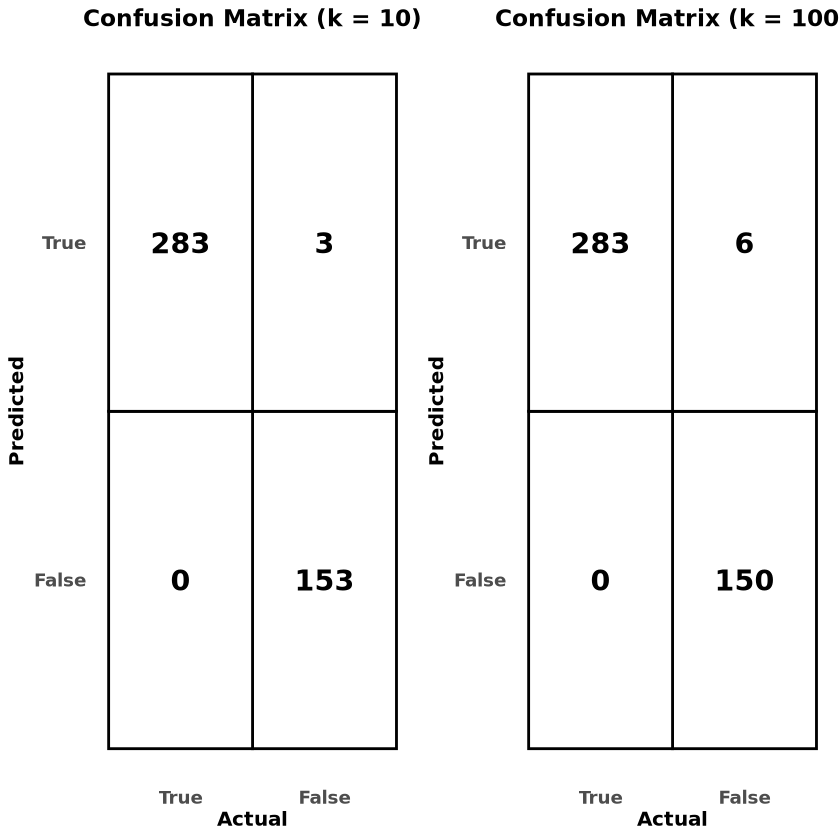
Prediction False True
False 153 0
True 3 283
Accuracy : 0.9932
95% CI : (0.9802, 0.9986)
No Information Rate : 0.6446
P-Value [Acc > NIR] : <2e-16
Kappa : 0.985
Mcnemar's Test P-Value : 0.2482
Sensitivity : 0.9808
Specificity : 1.0000
Pos Pred Value : 1.0000
Neg Pred Value : 0.9895
Prevalence : 0.3554
Detection Rate : 0.3485
Detection Prevalence : 0.3485
Balanced Accuracy : 0.9904
'Positive' Class : False
▶ 혼동행렬 (k = 100):
Confusion Matrix and Statistics
Reference
Prediction False True
False 150 0
True 6 283
Accuracy : 0.9863
95% CI : (0.9705, 0.995)
No Information Rate : 0.6446
P-Value [Acc > NIR] : < 2e-16
Kappa : 0.9699
Mcnemar's Test P-Value : 0.04123
Sensitivity : 0.9615
Specificity : 1.0000
Pos Pred Value : 1.0000
Neg Pred Value : 0.9792
Prevalence : 0.3554
Detection Rate : 0.3417
Detection Prevalence : 0.3417
Balanced Accuracy : 0.9808
'Positive' Class : False
- 그래프로 출력
# 혼동행렬 생성 <- confusionMatrix (best_pred, y_test)<- confusionMatrix (k100_pred, y_test)# 데이터프레임 변환 <- as.data.frame (cm_best$ table)<- as.data.frame (cm_k100$ table)# 열의 순서 (True → False) $ Reference <- factor (cm_best_df$ Reference, levels = c ("True" , "False" )) $ Reference <- factor (cm_k100_df$ Reference, levels = c ("True" , "False" ))
- 그래프 1 : 최적k 혼동행렬
<- ggplot (cm_best_df, aes (x = Reference, y = Prediction)) + geom_tile (fill = "white" , color = "black" , linewidth = 0.8 ) + geom_text (aes (label = Freq), size = 6 , fontface = "bold" ) + labs (title = paste0 ("Confusion Matrix (k = " , best_k, ")" ),x = "Actual" , y = "Predicted" ) + theme_minimal (base_family = "Helvetica" ) + theme (plot.title = element_text (size = 14 , face = "bold" , hjust = 0.5 ),axis.title = element_text (size = 12 , face = "bold" ),axis.text = element_text (size = 11 , face = "bold" ),panel.grid = element_blank (),legend.position = "none"
- 그래프 2 : k=100 혼동행렬
<- ggplot (cm_k100_df, aes (x = Reference, y = Prediction)) + geom_tile (fill = "white" , color = "black" , linewidth = 0.8 ) + geom_text (aes (label = Freq), size = 6 , fontface = "bold" ) + labs (title = "Confusion Matrix (k = 100)" ,x = "Actual" , y = "Predicted" ) + theme_minimal (base_family = "Helvetica" ) + theme (plot.title = element_text (size = 14 , face = "bold" , hjust = 0.5 ),axis.title = element_text (size = 12 , face = "bold" ),axis.text = element_text (size = 11 , face = "bold" ),panel.grid = element_blank (),legend.position = "none"
grid.arrange (p1, p2, nrow = 1 )