10. K-NN Regression

1. library

install.packages("FNN")

Updating HTML index of packages in '.Library'

Making 'packages.html' ...
 done

library(tidyverse)  # 데이터 처리 및 시각화
library(caret)      # 데이터 전처리, 모델링
library(FNN)        # KNN 회귀 함수 사용

2. Data

# 데이터 불러오기 (insurance.csv 파일 경로는 사용자 환경에 맞게 설정)
dt <- read.csv("insurance.csv")

# 기술통계
summary(dt)

      age            sex                 bmi           children    
 Min.   :18.00   Length:1338        Min.   :15.96   Min.   :0.000  
 1st Qu.:27.00   Class :character   1st Qu.:26.30   1st Qu.:0.000  
 Median :39.00   Mode  :character   Median :30.40   Median :1.000  
 Mean   :39.21                      Mean   :30.66   Mean   :1.095  
 3rd Qu.:51.00                      3rd Qu.:34.69   3rd Qu.:2.000  
 Max.   :64.00                      Max.   :53.13   Max.   :5.000  
    smoker             region             charges     
 Length:1338        Length:1338        Min.   : 1122  
 Class :character   Class :character   1st Qu.: 4740  
 Mode  :character   Mode  :character   Median : 9382  
                                       Mean   :13270  
                                       3rd Qu.:16640  
                                       Max.   :63770  

3. 전처리

- 범주형 변수 처리 및 범주형으로 변환

dt <- dt %>%
  mutate(
    sex = as.factor(sex),
    smoker = as.factor(smoker),
    region = as.factor(region)
  ) %>%
  mutate_if(is.factor, as.character) %>%   
  mutate_if(is.character, as.factor)       

- One-hot Encoding(fullRank=True로 다중공선성 방지)

dmy <- dummyVars(" ~ .", data = dt, fullRank = TRUE)
dt_transformed <- data.frame(predict(dmy, newdata = dt))

- 독립변수(X), 종속변수(y) 분리

X <- dt_transformed[, -which(names(dt_transformed) == "charges")]
y <- dt_transformed$charges

- 독립변수 표준화(평균0, 표준편차1)

4. 적합

pre_proc <- preProcess(X, method = c("center", "scale"))
X_scaled <- predict(pre_proc, X)

- 반복횟수 및 훈련 데이터 비율 설정

T <- 100                        # 100번 반복
N <- nrow(X_scaled)            # 전체 데이터 수
n_train <- round(0.7 * N)      # 70% 훈련 데이터

- 다양한 k값(1~100)에 대한 RMSE 저장 행렬 생성

k_range <- 1:100
rmse_matrix <- matrix(NA, nrow = T, ncol = length(k_range))  # (T x 100) 행렬

- 100번 반복하여 훈련/테스트 분할 및 RMSE 계산

for (t in 1:T) {
  set.seed(t)  # 반복마다 시드 고정
  train_idx <- sample(1:N, n_train, replace = FALSE)
  test_idx <- setdiff(1:N, train_idx)
  
  x_train <- X_scaled[train_idx, ]
  x_test <- X_scaled[test_idx, ]
  y_train <- y[train_idx]
  y_test <- y[test_idx]
  
  for (k in k_range) {
    # KNN 회귀 실행
    pred <- knn.reg(
      train = x_train,
      test = x_test,
      y = y_train,
      k = k
    )$pred
    
    # RMSE 계산 후 저장
    rmse <- sqrt(mean((y_test - pred)^2))
    rmse_matrix[t, k] <- rmse
  }
}

- k별 평균 RMSE 계산

avg_rmse <- colMeans(rmse_matrix, na.rm = TRUE)
results <- data.frame(k = k_range, RMSE = avg_rmse)

- RMSE 시각화

ggplot(results, aes(x = k, y = RMSE)) +
  geom_line(color = "steelblue", size = 1) +
  geom_point(color = "black") +
  labs(title = "K-NN Regression (100 different train/test splits)",
       x = "k",
       y = "Average RMSE") +
  theme_minimal()

Warning message:
“Using `size` aesthetic for lines was deprecated in ggplot2 3.4.0.
ℹ Please use `linewidth` instead.”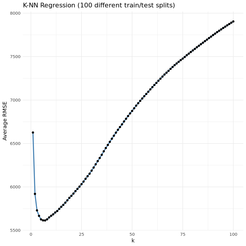

- 최적의 k 값 출력

best_k <- results$k[which.min(results$RMSE)]
cat("★ 최적의 k 값:", best_k, "\n")

★ 최적의 k 값: 7 

- 최종 예측 비교

set.seed(999)
train_index <- sample(1:N, n_train, replace = FALSE)
test_index <- setdiff(1:N, train_index)

- 최적 k로 예측

best_pred <- knn.reg(
  train = X_scaled[train_index, ],
  test = X_scaled[test_index, ],
  y = y[train_index],
  k = best_k
)

- k=100 으로 예측 (비교용)

k100_pred <- knn.reg(
  train = X_scaled[train_index, ],
  test = X_scaled[test_index, ],
  y = y[train_index],
  k = 100
)

- 예측값과 실제값의 상관계수 계산

cor_best <- cor(y[test_index], best_pred$pred)
cor_k100 <- cor(y[test_index], k100_pred$pred)

- 시각화

par(mfrow = c(1, 2))  # 1행 2열 그래프 레이아웃 설정

plot(y[test_index] ~ best_pred$pred,
     main = paste("k =", best_k),
     xlab = "Predicted Charges",
     ylab = "Actual Charges",
     col = "black", pch = 16)
abline(0, 1, col = rgb(1, 0, 0, alpha = 0.3), lwd = 2)
text(x = mean(range(best_pred$pred)),
     y = max(y[test_index]) * 0.95,
     labels = paste("Correlation =", round(cor_best, 3)),
     col = "black", cex = 1.2, font = 1)
legend("topleft",
       legend = "y = x",
       col = rgb(1, 0, 0, 0.3),
       lty = 1,
       lwd = 2,
       bty = "n")

plot(y[test_index] ~ k100_pred$pred,
     main = "k = 100",
     xlab = "Predicted Charges",
     ylab = "Actual Charges",
     col = "black", pch = 16)
abline(0, 1, col = rgb(1, 0, 0, alpha = 0.3), lwd = 2)
text(x = mean(range(k100_pred$pred)),
     y = max(y[test_index]) * 0.95,
     labels = paste("Correlation =", round(cor_k100, 3)),
     col = "black", cex = 1.2, font = 1)
legend("topleft",
       legend = "y = x",
       col = rgb(1, 0, 0, 0.3),
       lty = 1,
       lwd = 2,
       bty = "n")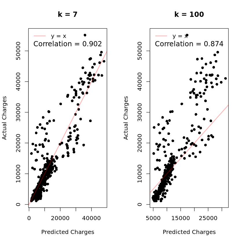

---

- 레이아웃 초기화

par(mfrow = c(1, 1))