# install.packages("ggplot2")
library(ggplot2)1. imports
2. data
data(diamonds)- cut, color, clarity를 범주형(factor)로 변환
diamonds$cut <- factor(diamonds$cut, ordered = FALSE)
diamonds$color <- factor(diamonds$color, ordered = FALSE)
diamonds$clarity <- factor(diamonds$clarity, ordered = FALSE)
- 사용할 변수 선택
diamonds_sub <- diamonds[, c("price", "carat", "cut", "color", "clarity", "depth", "table", "x", "y", "z")]- 데이터 셔플
set.seed(2025)  # 재현성 확보
shuffled_idx <- sample(nrow(diamonds_sub))
diamonds_sub <- diamonds_sub[shuffled_idx, ]
- 데이터 분할(70% train, 30% test)
n <- nrow(diamonds_sub)
n_train <- round(0.7 * n)
train_data <- diamonds_sub[1:n_train, ]
test_data <- diamonds_sub[(n_train + 1):n, ]3. 모델 학습
model <- lm(price ~ carat + cut + color + clarity + depth + table + x + y + z, data = train_data)summary(model)
Call:
lm(formula = price ~ carat + cut + color + clarity + depth +
    table + x + y + z, data = train_data)

Residuals:
     Min       1Q   Median       3Q      Max
-21193.1   -592.3   -184.2    379.4  10019.2

Coefficients:
              Estimate Std. Error t value Pr(>|t|)
(Intercept)   2523.821    486.284   5.190 2.11e-07 ***
carat        11166.722     57.804 193.183  < 2e-16 ***
cutGood        569.597     40.501  14.064  < 2e-16 ***
cutVery Good   708.343     38.926  18.197  < 2e-16 ***
cutPremium     752.076     38.947  19.310  < 2e-16 ***
cutIdeal       810.282     40.340  20.086  < 2e-16 ***
colorE        -207.868     21.473  -9.681  < 2e-16 ***
colorF        -253.152     21.671 -11.681  < 2e-16 ***
colorG        -476.298     21.273 -22.390  < 2e-16 ***
colorH        -967.243     22.517 -42.956  < 2e-16 ***
colorI       -1462.027     25.326 -57.728  < 2e-16 ***
colorJ       -2379.519     31.042 -76.655  < 2e-16 ***
claritySI2    2660.652     51.379  51.784  < 2e-16 ***
claritySI1    3638.154     51.113  71.179  < 2e-16 ***
clarityVS2    4247.626     51.407  82.627  < 2e-16 ***
clarityVS1    4551.296     52.258  87.093  < 2e-16 ***
clarityVVS2   4918.192     53.839  91.350  < 2e-16 ***
clarityVVS1   4987.707     55.359  90.097  < 2e-16 ***
clarityIF     5297.251     59.893  88.445  < 2e-16 ***
depth          -69.236      5.335 -12.979  < 2e-16 ***
table          -28.518      3.496  -8.157 3.55e-16 ***
x             -964.321     35.990 -26.794  < 2e-16 ***
y               -2.101     19.444  -0.108    0.914
z              -40.404     35.011  -1.154    0.248
---
Signif. codes:  0 ‘***’ 0.001 ‘**’ 0.01 ‘*’ 0.05 ‘.’ 0.1 ‘ ’ 1

Residual standard error: 1129 on 37734 degrees of freedom
Multiple R-squared:  0.9198,    Adjusted R-squared:  0.9197
F-statistic: 1.881e+04 on 23 and 37734 DF,  p-value: < 2.2e-16
4. 모델 평가
- test_set 예측
test_pred <- predict(model, newdata = test_data)- test 성능 평가(RMSE 계산)
test_rmse <- sqrt(mean((test_pred - test_data$price)^2))
cat("Test RMSE:", round(test_rmse, 2), "\n")
Test RMSE: 1132.54 - 예측 vs 실제 산점도 (test set)
plot(test_pred, test_data$price,
     xlab = "Predicted Price", ylab = "Actual Price",
     main = "Test Set: Predicted vs Actual Price",
     pch = 16, col = "blue")
abline(0, 1, col = "red", lwd = 2)  # 완벽한 예측선 (y = x)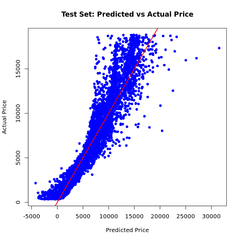
- RMSE값 그래프에 추가
text(x = max(test_pred) * 0.7,
     y = min(test_data$price) * 1.2,
     labels = paste0("Test RMSE = ", round(test_rmse, 2)),
     pos = 4,
     col = "black",
     cex = 0.9)
ERROR: Error in text.default(x = max(test_pred) * 0.7, y = min(test_data$price) * : plot.new has not been called yet
Error in text.default(x = max(test_pred) * 0.7, y = min(test_data$price) * : plot.new has not been called yet
Traceback:
1. text(x = max(test_pred) * 0.7, y = min(test_data$price) * 1.2,
. labels = paste0("Test RMSE = ", round(test_rmse, 2)), pos = 4,
. col = "black", cex = 0.9)
2. text.default(x = max(test_pred) * 0.7, y = min(test_data$price) *
. 1.2, labels = paste0("Test RMSE = ", round(test_rmse, 2)),
. pos = 4, col = "black", cex = 0.9)- 새로운 데이터 생성
new_data <- data.frame(
  carat = c(0.5, 1.2),
  cut = factor(c("Ideal", "Premium"), levels = levels(diamonds$cut)),
  color = factor(c("E", "H"), levels = levels(diamonds$color)),
  clarity = factor(c("VS2", "SI1"), levels = levels(diamonds$clarity)),
  depth = c(61.5, 62.2),
  table = c(55, 58),
  x = c(5.1, 6.9),
  y = c(5.2, 7.1),
  z = c(3.15, 4.35)
)
- 새로운 데이터 예측 및 결과 출력
predicted_prices <- predict(model, newdata = new_data)new_data$predicted_price <- round(predicted_prices, 2)
new_data| carat | cut | color | clarity | depth | table | x | y | z | predicted_price |
|---|---|---|---|---|---|---|---|---|---|
| <dbl> | <fct> | <fct> | <fct> | <dbl> | <dbl> | <dbl> | <dbl> | <dbl> | <dbl> |
| 0.5 | Ideal | E | VS2 | 61.5 | 55 | 5.1 | 5.2 | 3.15 | 2074.45 |
| 1.2 | Premium | H | SI1 | 62.2 | 58 | 6.9 | 7.1 | 4.35 | 6541.83 |