import numpy as npimport matplotlib.pyplot as pltimport seaborn as snsfrom scipy.stats import skewnormdef simulate_clt(distribution_type, sample_size, num_samples, **kwargs):""" 중심극한정리(CLT) 시뮬레이션 함수 Args: distribution_type (str): 모집단 분포 종류 ('uniform', 'exponential', 'normal', 'skewed_left', 'skewed_right') sample_size (int): 각 표본의 크기 num_samples (int): 표본의 개수 **kwargs: 각 분포에 따른 추가 매개변수 - uniform: low (default=0), high (default=1) - exponential: scale (default=1) (scale = 1/lambda) - normal: loc (default=0), scale (default=1) (loc: 평균, scale: 표준편차) - binomal: (n, p) - gamma: (shape, scale) Returns: None (히스토그램 시각화) """ sample_means = []for _ inrange(num_samples):if distribution_type =='uniform': sample = np.random.uniform(low=kwargs.get('low', 0), high=kwargs.get('high', 1), size=sample_size)elif distribution_type =='exponential': sample = np.random.exponential(scale=kwargs.get('scale', 1), size=sample_size)elif distribution_type =='normal': sample = np.random.normal(loc=kwargs.get('loc', 0), scale=kwargs.get('scale', 1), size=sample_size)elif distribution_type =='binomial': sample = np.random.binomial(kwargs.get('n', 100), kwargs.get('p', 0.5), size=sample_size)elif distribution_type =='gamma': sample = np.random.gamma(3, 2, size=sample_size)else:raiseValueError("Invalid distribution type.") sample_means.append(np.mean(sample)) plt.figure(figsize=(8, 6)) sns.histplot(sample_means, kde=True, stat="density") plt.title(f"Distribution of Sample Means (n={sample_size}, {num_samples} samples)\nFrom {distribution_type} distribution", fontsize=14) plt.xlabel("Sample Mean", fontsize=12) plt.ylabel("Density", fontsize=12) plt.show()return sample_means# 실험 설정distributions = {# 'uniform': {'low': 0, 'high': 1},# 'exponential': {'scale': 1},# 'normal': {'loc': 0, 'scale': 1},# 'binomial': {'n': 100, 'p': 0.1},'gamma': {'shape': 3, 'scale': 2},}sample_sizes = [5, 100, 1000]num_samples_list = [1000]# 다양한 분포, 표본 크기, 표본 개수에 대한 실험for dist_name, dist_params in distributions.items():for sample_size in sample_sizes:for num_samples in num_samples_list:print(f"\n--- {dist_name}, sample_size={sample_size}, num_samples={num_samples} ---") simulate_clt(dist_name, sample_size, num_samples, **dist_params)
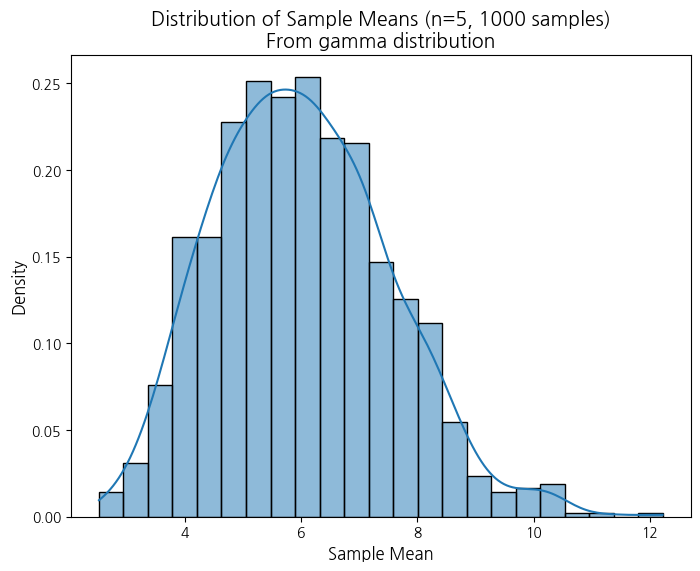
--- gamma, sample_size=5, num_samples=1000 ---
/root/anaconda3/envs/pypy/lib/python3.10/site-packages/seaborn/_oldcore.py:1119: FutureWarning: use_inf_as_na option is deprecated and will be removed in a future version. Convert inf values to NaN before operating instead.
  with pd.option_context('mode.use_inf_as_na', True):
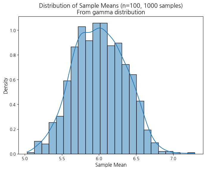
--- gamma, sample_size=100, num_samples=1000 ---
/root/anaconda3/envs/pypy/lib/python3.10/site-packages/seaborn/_oldcore.py:1119: FutureWarning: use_inf_as_na option is deprecated and will be removed in a future version. Convert inf values to NaN before operating instead.
  with pd.option_context('mode.use_inf_as_na', True):
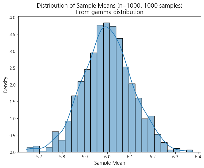
--- gamma, sample_size=1000, num_samples=1000 ---
/root/anaconda3/envs/pypy/lib/python3.10/site-packages/seaborn/_oldcore.py:1119: FutureWarning: use_inf_as_na option is deprecated and will be removed in a future version. Convert inf values to NaN before operating instead.
  with pd.option_context('mode.use_inf_as_na', True):
- 정규분포라고 하기에는 약간 애매
분포를 바꿔가면서 할 수 있음!!!
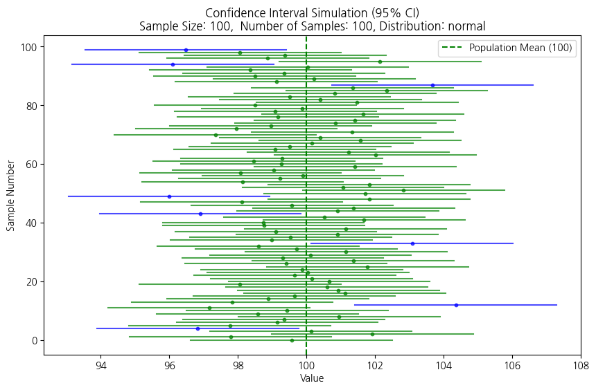
2. Simulation for Confidence Interval
import numpy as npimport matplotlib.pyplot as pltfrom scipy.stats import norm, t # 정규분포, t-분포 사용def confidence_interval_simulation(population_mean, population_std, sample_size, num_samples, confidence_level=0.95, distribution='normal'):""" 신뢰구간 시뮬레이션 함수 Args: population_mean (float): 모집단 평균 population_std (float): 모집단 표준편차 sample_size (int): 표본 크기 num_samples (int): 표본 추출 횟수 (시뮬레이션 반복 횟수) confidence_level (float): 신뢰 수준 (default: 0.95) distribution (str): 'normal' (정규분포) 또는 't' (t-분포) (default: 'normal') Returns: None (신뢰구간 시각화 및 포함 비율 출력) """if distribution notin ['normal', 't']:raiseValueError("distribution must be 'normal' or 't'") intervals_containing_mean =0# 모집단 평균을 포함하는 신뢰구간 개수 plt.figure(figsize=(10, 6))for _ inrange(num_samples):# 1. 표본 추출 sample = np.random.normal(loc=population_mean, scale=population_std, size=sample_size) sample_mean = np.mean(sample) sample_std = np.std(sample, ddof=1) # 표본 표준편차 (불편추정량, ddof=1)# 2. 신뢰구간 계산if distribution =='normal':# 정규분포 기반 (모집단 표준편차를 알 때) z_critical = norm.ppf((1+ confidence_level) /2) # Z-critical value margin_of_error = z_critical * (population_std / np.sqrt(sample_size)) lower_bound = sample_mean - margin_of_error upper_bound = sample_mean + margin_of_errorelse: # distribution == 't'# t-분포 기반 (모집단 표준편차를 모를 때) t_critical = t.ppf((1+ confidence_level) /2, df=sample_size -1) # t-critical value margin_of_error = t_critical * (sample_std / np.sqrt(sample_size)) # 표본표준편차 사용 lower_bound = sample_mean - margin_of_error upper_bound = sample_mean + margin_of_error# 3. 신뢰구간이 모집단 평균을 포함하는지 확인if lower_bound <= population_mean <= upper_bound: intervals_containing_mean +=1 color ='green'# 포함하면 파란색else: color ='blue'# 포함하지 않으면 빨간색# 4. 신뢰구간 시각화 plt.plot([lower_bound, upper_bound], [_, _], color=color, alpha=0.7) plt.scatter(sample_mean, _, color=color, s=10, alpha=0.7) # 표본평균 표시# 5. 결과 출력 plt.axvline(x=population_mean, color='green', linestyle='--', label=f'Population Mean ({population_mean})') # 모집단 평균 (녹색 점선) plt.title(f"Confidence Interval Simulation ({confidence_level*100:.0f}% CI)\n"f"Sample Size: {sample_size}, Number of Samples: {num_samples}, Distribution: {distribution}") plt.xlabel("Value") plt.ylabel("Sample Number") plt.legend() plt.show() inclusion_rate = (intervals_containing_mean / num_samples) *100print(f"Inclusion Rate: {inclusion_rate:.2f}% ({intervals_containing_mean} out of {num_samples} intervals contained the population mean)")# 시뮬레이션 실행 예시population_mean =100# 모집단 평균population_std =15# 모집단 표준편차sample_size =100# 표본 크기num_samples =100# 표본 추출 횟수# 정규분포 기반 신뢰구간 시뮬레이션confidence_interval_simulation(population_mean, population_std, sample_size, num_samples, confidence_level=0.95, distribution='normal')# t-분포 기반 신뢰구간 시뮬레이션 (모표준편차 모를 때)#confidence_interval_simulation(population_mean, population_std, sample_size, num_samples, confidence_level=0.95, distribution='t')
Inclusion Rate: 92.00% (92 out of 100 intervals contained the population mean)
- 코드는 몰라도 됨
결과에 대한 분석만 할 줄 알면 됨
confidence_level 바꿔가며 실험
표본크기 바꿔가며 실험 \(\to\) 표본 크기에 따라 양상이 달라짐
3. Example of indep. two sample t.test
import pandas as pdfrom scipy.stats import ttest_indimport numpy as np# 1. 데이터 불러오기 및 확인# CSV 파일 읽기df = pd.read_csv("GG.csv")print("원본 데이터:\n", df)# 2. 데이터 분리 및 결측치 처리# male, female 데이터를 각각 NumPy 배열로 변환male_height = df['male'].to_numpy()female_height = df['female'].to_numpy()# NumPy의 isnan() 함수를 사용하여 NaN 값 제거male_height_cleaned = male_height[~np.isnan(male_height)].astype(float)female_height_cleaned = female_height[~np.isnan(female_height)].astype(float)print("\n결측치 제거 후 male 키 데이터:\n", male_height_cleaned)print("\n결측치 제거 후 female 키 데이터:\n", female_height_cleaned)# 3. 독립표본 t-검정 (등분산 가정)# 귀무가설 (H0): 남학생 키의 모평균과 여학생 키의 모평균은 같다. (모분산 같음)# 대립가설 (H1): 남학생 키의 모평균과 여학생 키의 모평균은 다르다.# equal_var=True (등분산 가정)t_stat_equal, p_val_equal = ttest_ind(male_height_cleaned, female_height_cleaned, equal_var=True)print("\n--- 등분산 가정 t-검정 ---")print("t-statistic:", t_stat_equal)print("p-value:", p_val_equal)# 결과 해석 (등분산 가정)alpha =0.05# 유의 수준if p_val_equal < alpha:print("등분산 가정: 귀무가설 기각 - 남녀 키 평균은 통계적으로 유의미하게 다릅니다.")else:print("등분산 가정: 귀무가설 채택 - 남녀 키 평균은 통계적으로 유의미한 차이가 없습니다.")# 4. 독립표본 t-검정 (이분산 가정)# 귀무가설 (H0): 남학생 키의 모평균과 여학생 키의 모평균은 같다. (모분산 다름)# 대립가설 (H1): 남학생 키의 모평균과 여학생 키의 모평균은 다르다.# equal_var=False (이분산 가정, Welch's t-test)t_stat_welch, p_val_welch = ttest_ind(male_height_cleaned, female_height_cleaned, equal_var=False)print("\n--- 이분산 가정 t-검정 (Welch's t-test) ---")print("t-statistic:", t_stat_welch)print("p-value:", p_val_welch)# 결과 해석 (이분산 가정)if p_val_welch < alpha:print("이분산 가정: 귀무가설 기각 - 남녀 키 평균은 통계적으로 유의미하게 다릅니다.")else:print("이분산 가정: 귀무가설 채택 - 남녀 키 평균은 통계적으로 유의미한 차이가 없습니다.")#### 참고사항: scipy 버전에 따라 자유도가 출력될 수 있음: 각자의 컴퓨터마다 아래 결과에 "df ="출력될 수 있으니 돌려보기만 하면 됩니다.print(ttest_ind(male_height_cleaned, female_height_cleaned, equal_var=True))print(ttest_ind(male_height_cleaned, female_height_cleaned, equal_var=False))
원본 데이터:
     male  female
0    114   108.0
1     96    98.0
2     80    88.0
3    102    86.0
4     94   100.0
5     94    98.0
6     98   104.0
7     92   102.0
8     94    94.0
9    100     NaN
10   108     NaN
11   110     NaN
12    90     NaN
13    90     NaN
14    82     NaN
15   106     NaN

결측치 제거 후 male 키 데이터:
 [114.  96.  80. 102.  94.  94.  98.  92.  94. 100. 108. 110.  90.  90.
  82. 106.]

결측치 제거 후 female 키 데이터:
 [108.  98.  88.  86. 100.  98. 104. 102.  94.]

--- 등분산 가정 t-검정 ---
t-statistic: -0.18597961132240054
p-value: 0.8540912649163084
등분산 가정: 귀무가설 채택 - 남녀 키 평균은 통계적으로 유의미한 차이가 없습니다.

--- 이분산 가정 t-검정 (Welch's t-test) ---
t-statistic: -0.20139794503778663
p-value: 0.8423466136276512
이분산 가정: 귀무가설 채택 - 남녀 키 평균은 통계적으로 유의미한 차이가 없습니다.
TtestResult(statistic=-0.18597961132240054, pvalue=0.8540912649163084, df=23.0)
TtestResult(statistic=-0.20139794503778663, pvalue=0.8423466136276512, df=20.771503751242072)