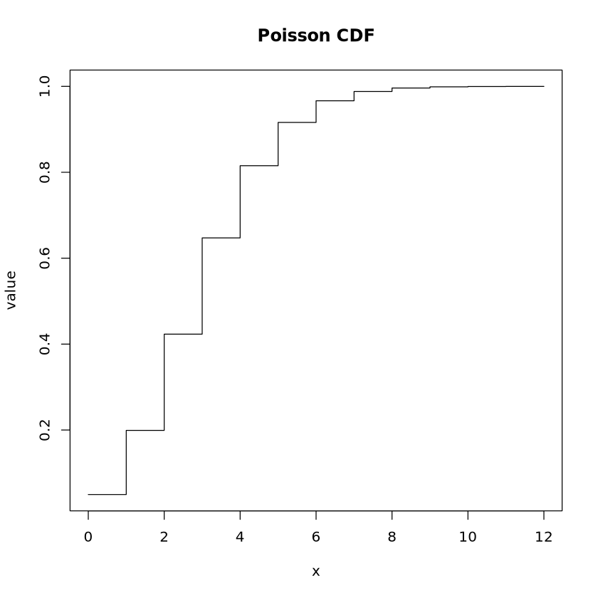
poisson_quantile <-qpois(p =0.9, lambda =3)print("Poisson Quantile at p=0.9:")print(poisson_quantile)
[1] "Poisson Quantile at p=0.9:"
[1] 5
- 추가
- 감마 분포
평균 : \(\alpha\) x \(\beta\)
분산 : \(\alpha\) x \(\beta^2\)
mean(rgamma(100000,1,3))var(rgamma(100000,1,3))
0.333018431858545
0.111819570741366
-ggplot
library(ggplot2)library(tidyr)
results <-data.frame(Distribution =character(),Value =numeric(),Type =character(), # Mean, Median, Variance를 구분하는 열 추가stringsAsFactors =FALSE)
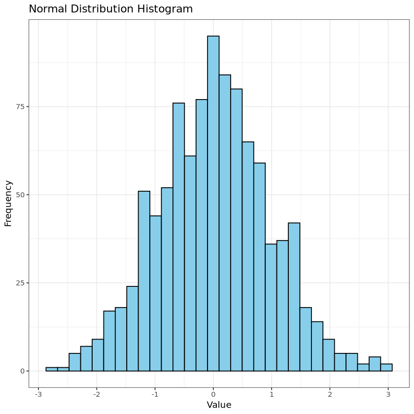
# 1. Normal Distributionnormal_data <-rnorm(n =1000, mean =0, sd =1)
# ggplot histogram ggplot(data.frame(Value = normal_data), aes(x = Value)) +geom_histogram(bins =30, fill ="skyblue", color ="black") +# bins: 막대 개수labs(title ="Normal Distribution Histogram", x ="Value", y ="Frequency") +theme_bw()
# results results <-rbind(results,data.frame(Distribution ="Normal", Value =mean(normal_data), Type ="Mean"),data.frame(Distribution ="Normal", Value =median(normal_data), Type ="Median"),data.frame(Distribution ="Normal", Value =var(normal_data), Type ="Variance"))
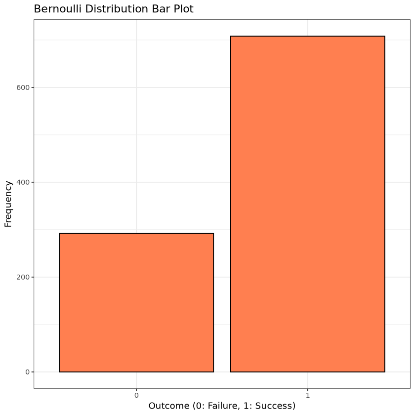
# ggplot bar plot ggplot(data.frame(Outcome =factor(bernoulli_data)), aes(x = Outcome)) +geom_bar(fill ="coral", color ="black") +labs(title ="Bernoulli Distribution Bar Plot", x ="Outcome (0: Failure, 1: Success)", y ="Frequency") +theme_bw()
results <-rbind(results,data.frame(Distribution ="Bernoulli", Value =mean(bernoulli_data), Type ="Mean"),data.frame(Distribution ="Bernoulli", Value =median(bernoulli_data), Type ="Median"),data.frame(Distribution ="Bernoulli", Value =var(bernoulli_data), Type ="Variance"))
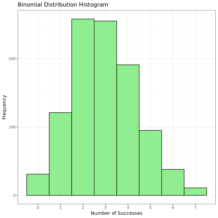
# ggplot histogram ggplot(data.frame(Successes = binomial_data), aes(x = Successes)) +geom_histogram(binwidth =1, fill ="lightgreen", color ="black") +# binwidth: 막대 너비labs(title ="Binomial Distribution Histogram", x ="Number of Successes", y ="Frequency") +scale_x_continuous(breaks =seq(0, 10, by =1)) +# x축 눈금 설정theme_bw()
results <-rbind(results,data.frame(Distribution ="Binomial", Value =mean(binomial_data), Type ="Mean"),data.frame(Distribution ="Binomial", Value =median(binomial_data), Type ="Median"),data.frame(Distribution ="Binomial", Value =var(binomial_data), Type ="Variance"))
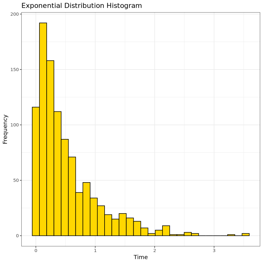
# ggplot histogram ggplot(data.frame(Time = exponential_data), aes(x = Time)) +geom_histogram(bins =30, fill ="gold", color ="black") +labs(title ="Exponential Distribution Histogram", x ="Time", y ="Frequency") +theme_bw()
results <-rbind(results,data.frame(Distribution ="Exponential", Value =mean(exponential_data), Type ="Mean"),data.frame(Distribution ="Exponential", Value =median(exponential_data), Type ="Median"),data.frame(Distribution ="Exponential", Value =var(exponential_data), Type ="Variance"))
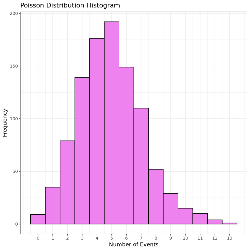
# ggplot histogram ggplot(data.frame(Events = poisson_data), aes(x = Events)) +geom_histogram(binwidth =1, fill ="violet", color ="black") +labs(title ="Poisson Distribution Histogram", x ="Number of Events", y ="Frequency") +scale_x_continuous(breaks =seq(0, max(poisson_data), by =1)) +theme_bw()
results <-rbind(results,data.frame(Distribution ="Poisson", Value =mean(poisson_data), Type ="Mean"),data.frame(Distribution ="Poisson", Value =median(poisson_data), Type ="Median"),data.frame(Distribution ="Poisson", Value =var(poisson_data), Type ="Variance"))